
Understanding AR Model with Statsmodels: A Detailed Guide for You
Are you intrigued by the world of time series analysis and looking to delve into the autoregressive (AR) model? If so, you’ve come to the right place. In this article, I’ll walk you through the ins and outs of the AR model using the popular Python library, Statsmodels. By the end, you’ll have a comprehensive understanding of how to build, interpret, and evaluate AR models.
What is an AR Model?

An autoregressive model, often referred to as an AR model, is a type of time series model that uses past observations to predict future values. The key idea behind an AR model is that the future values of a variable are dependent on its past values. This makes AR models particularly useful for analyzing data that exhibit temporal dependencies, such as stock prices, weather patterns, or sales figures.
Statsmodels: Your Go-To Library
Statsmodels is a powerful Python library that provides a wide range of statistical models, including AR models. With Statsmodels, you can easily fit, predict, and evaluate AR models for your time series data. Let’s dive into how to use Statsmodels to build an AR model.
Step-by-Step Guide to Building an AR Model with Statsmodels
Here’s a step-by-step guide to building an AR model using Statsmodels:
-
Import the necessary libraries:
import pandas as pdimport numpy as npfrom statsmodels.tsa.ar_model import AutoReg -
Load your time series data:
data = pd.read_csv('your_data.csv', index_col='date', parse_dates=True) -
Split your data into training and testing sets:
train_size = int(len(data) 0.8)train, test = data[0:train_size], data[train_size:len(data)] -
Fit the AR model to your training data:
model = AutoReg(train, lags=5)model_fit = model.fit(disp=0) -
Make predictions on your testing data:
predictions = model_fit.predict(start=len(train), end=len(train) + len(test) - 1, dynamic=True) -
Evaluate the model’s performance:
from sklearn.metrics import mean_squared_errormse = mean_squared_error(test, predictions)print('Mean Squared Error:', mse)
Interpreting the Results
Once you’ve built and evaluated your AR model, it’s important to interpret the results. Here are some key points to consider:
-
Model Parameters:
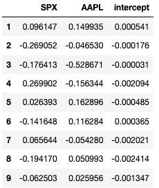
The parameters of the AR model, such as the lag order and the coefficients, provide insights into the relationships between past and future values. For example, a high coefficient for a particular lag suggests that past values have a strong influence on future values.
-
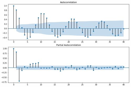
Residuals:
The residuals of the AR model represent the difference between the observed values and the predicted values. By analyzing the residuals, you can identify patterns or anomalies in your data that may not be captured by the model.
-
Model Fit:
The overall fit of the AR model can be assessed using various metrics, such as the mean squared error (MSE) or the adjusted R-squared value. A lower MSE or a higher adjusted R-squared value indicates a better fit.
Case Study: Stock Price Prediction
Let’s consider a practical example of using an AR model to predict stock prices. We’ll use historical stock price data for a popular company and build an AR model to forecast future prices.
| Date | Stock Price |
|---|---|
| 2020-01-01 | 100.00 |
| 2020-01-02 | 101.50 |


